Conditional formatting in Google Sheets
Notes
- The conditional formatting rules are processed in order. You can adjust the order of the rules by dragging the three dots that appear when you hover over the rule
- You can negate a statement with
NOT(). For exampleNOT(ISBLANK())will look up non-empty values - You can check for multiple conditions with
AND(value1, value2, value3)
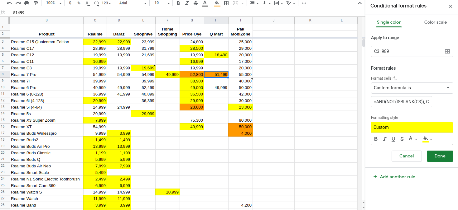
Highlight prices that are lower than reference price
=(AND(NOT(ISBLANK(D3)), D3<$C3))
- Highlights all cells that have price lower than the official price column.
- Only highlights non-empty cells
C3 vs $C3
$C3 will keep the column constant. otherwise it kept comparing later columns with the immediately next neighbour instead of column C. (comparing E with D, F with E, G with F and so on instead of comparing them all to C)
$C$3- keep row and column constant, i.e. this particular cell only, don't adjust thisC$3- keep row constant$C3- keep column constant
Highlight the lowest value in row
=C3=MIN($C3:$I3)
=AND(NOT(ISBLANK(C3)), C3=MIN($C3:$I3))
Navigate to conditional formatting. Set the conditional formatting range to include all the values you are checking
In the custom formula field, enter
=A1=MIN($A1:$N1). SubstituteA1for the first cell in the first row you are checking, andN1with the last cell in the first row you are checking.